11. Non-normal data
This session is about checking whether the assumptions of normality and equal variance hold and what to do when they don’t: non-parametric tests.
What Does “Normally Distributed” Mean Here?
When we say a dataset is normally distributed for the purposes of a parametric test, we mean that the data were randomly sampled from a normally distributed population; not that the sample itself looks perfectly normal.
This is an important distinction: a small sample from a normal population will rarely look like a clean bell curve. What matters is whether the assumption of normality is plausible for the underlying data-generating process and whether the sample data represents that normal distribution well.
Checking Normality
Visual methods:
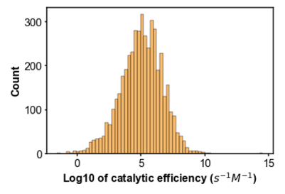
A histogram or violin plot can provide a rough check. Look for approximate symmetry and a single peak (but with small n, even normal data will not look bell-shaped).
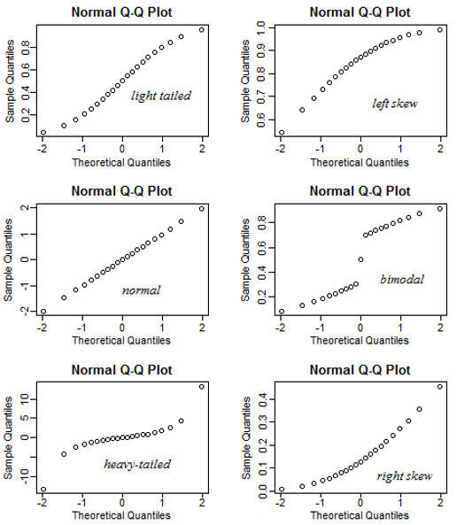
A Q-Q plot compares your data’s quantiles to a normal distribution’s: points on a straight diagonal mean approximately normal; S-curves suggest heavy/light tails, arcs suggest skew.
Let’s load some data that contain several conditions with different spreads and first inspect visually:
These visual tests are subjective, and with small sample sizes can be very difficult to assess.
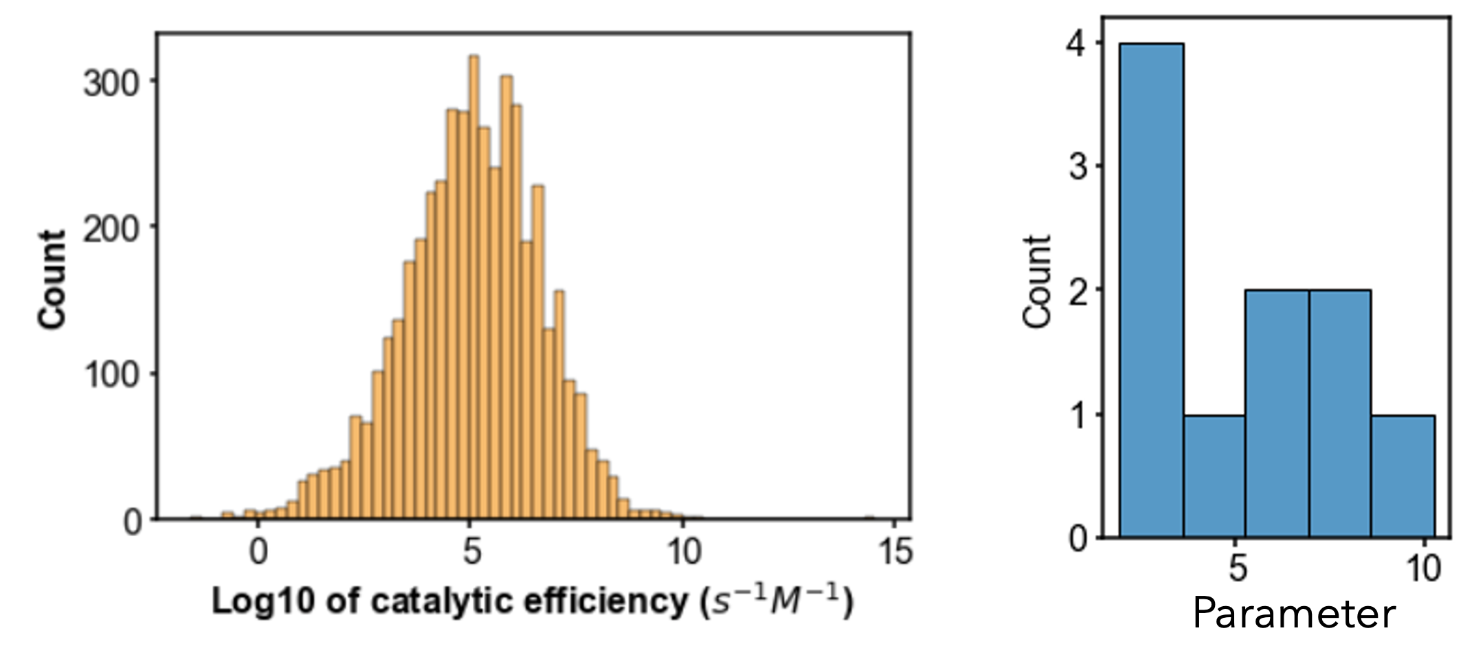
Is there a way that we can make more objective assessments? Yes!
The Shapiro-Wilk test evaluates the null hypothesis that the data came from a normal distribution: p > 0.05 → cannot reject normality (proceed parametric); p < 0.05 → reject (go non-parametric).
Shapiro-Wilk caveats: at small n (< 5–10) it has very low power (rarely rejects even clearly non-normal data); at large n (> 100–200) it has so much power it flags trivial, irrelevant deviations. It is most useful for n ≈ 10–50; at the extremes, it is advisable to include domain knowledge and the Q-Q plot.
Checking Variance Equality (Homoscedasticity)
If the data are normal, the next question is whether the groups have similar variances.
- Bartlett’s test is standard for normal data;
- Levene’s test is more robust when normality is uncertain.
If the data are normal but heteroscedastic (unequal variances), apply the Welch correction:
\[t_{\text{Welch}} = \frac{\bar{x}_1 - \bar{x}_2}{\sqrt{\frac{s_1^2}{n_1} + \frac{s_2^2}{n_2}}}\]
The Welch correction adjusts the degrees of freedom for unequal variances; it is also appropriate when the two groups have different sample sizes, even if variances are equal. (In pingouin.ttest, correction="auto" applies it automatically — Session 8.)
Non-Parametric Tests
When data are not normally distributed, non-parametric tests are used (regardless of homoscedasticity). Instead of directly using measured values, non-parametric tests evaluate ranked data.
Converting data to ranks discards information about the magnitude of differences: you only know that one value is larger than another, not by how much. This is why non-parametric tests have lower statistical power than their parametric equivalents. However, when the normality assumption is strongly violated, p-values derived from parametric tests can be unreliable. A valid, lower-powered test is preferable to an invalid, higher-powered one.
| Parametric | Non-parametric | Use case |
|---|---|---|
| Independent t-test | Mann-Whitney U | Two independent groups |
| Paired t-test | Wilcoxon signed-rank | Two paired measurements |
| One-way ANOVA | Kruskal-Wallis | Three or more independent groups |
- Mann-Whitney U tests whether one group’s median differs from another’s.
- Wilcoxon signed-rank is the paired version (same sample measured twice).
- Kruskal-Wallis generalizes to three or more independent groups.
What about the effect size for these non-parametric tests?
A standard effect size for these three non-parametric tests is the Common Language Effect Size (CLES). The CLES gives the probability a random value from A exceeds a random value from B. A CLES value of 0.5 (or 50%) indicates no effect. Values closer to 0 or 1 have larger effects. In pingouin, the effect size for the non-parametric tests can requested with eftype="CLES" in pg.compute_effsize.
Often students are confused: why would we even perform a Levene’s test if there is no homoscedasticity correction for non-parameteric tests?
While Bartlett is to assess if modifications to a subsequent test are necessary, Levene’s test is to directly evaluate homoscedasticity.
Maybe your research question is Which method yields a lower variance in outcome? Then you need a statistical method to evaluate a null hypothesis related directly to comparing variance. If your data is normally distributed, use Barlett’s test, and if the data is non-normally distributed, use Levene’s test.
Non-parametric tests and Power
Power calculations for non-parametric tests require explicit assumptions about the underlying distribution. Without those assumptions, true sample size calculations are impossible. A common rule of thumb is that non-parametric analyses require approximately 15% larger sample sizes than equivalent parametric analyses, but this is a rough approximation and should not replace formal power analysis when it is feasible.
An Overall Statistical Analysis Workflow when x is discrete or categorical data
How do these evaluations fit into a statistical analysis workflow? A typical workflow is provided below.
- Define research question and hypotheses
- Design the experiment (controls and replicates)
- Collect the data
- Visualize the data and transform if necessary*
- Determine descriptive statistics and error metrics
- Assess normality
- If normal, test variance. If non-normal, test for outliers (if any are removed, re-assess normality and variance, but do NOT detect outliers again)*
- Assess inferential statistics (including power and effect size)
- Visualize data with inferential statistics
- Formulate conclusions
- Report methods, results, and conclusions
*We will discuss transformations and outliers next week!
Warning on mis-use of statistics
Once you have chosen a statistical test based on your data type and distribution, do not change the test after seeing the results. Using the Mann-Whitney test, finding a non-significant result, and then switching to a t-test because it gives p < 0.05 is a form of significance chasing (or p-hacking).
A specific example: for non-normally distributed data, the Mann-Whitney test correctly returns a non-significant result (\(\alpha\) = 0.050, p = 0.055). The t-test, applied to the same data, returns a significant result (\(\alpha\) = 0.050, p = 0.029). If you select the t-test result because it supports your hypothesis, you have effectively found a 50/50 vote and picked the result you preferred. This is an example of both p-hacking and cherry-picking. The pre-specified test (Mann-Whitney, appropriate for non-normal data) is the correct analysis; the t-test result is irrelevant.
Please note: in the exam, logic that relies on p-hacking will result in zero points for the question.
Further Reading
- 10.3758/s13428-021-01587-5 — on how much the normality assumption matters in practice
- https://www.itl.nist.gov/div898/handbook/eda/section3/eda35.htm — NIST resource on normality and variance tests
- Check normality (Q-Q plot, Shapiro–Wilk — unreliable at very small/large n) and variance (Bartlett/Levene).
- Normal but unequal variances → apply the Welch correction.
- Non-normal → non-parametric tests (Mann–Whitney, Wilcoxon, Kruskal–Wallis): rank-based, lower power but valid.
- Pre-specify the test; switching tests to chase significance is p-hacking.
- In Python:
pg.normality(...),pg.homoscedasticity(..., method=),pg.mwu(...),pg.wilcoxon(...),pg.kruskal(...).
In Person
TBD