12. Outliers and Transformations

Updated

October 5, 2026

This session covers outliers and transformations, applied in Python with pingouin and scikit-learn.

Identifying Outliers

An outlier is an observation that is unusually far from the rest of the data. Outliers require careful treatment: they should only be removed with a clear, documented justification. They should not simply because they are inconvenient!

Legitimate reasons to remove an outlier: - Gross error (confirmed equipment failure, contamination, transcription error) - Significant reason to believe there was a measurement error at that specific point - The observation is the result of an uncontrolled factor that was identified independently

Methods for Identifying Outliers

Visual inspection: histogram or Q-Q plot — look for isolated points far from the main distribution.

Inner fence method: \[\text{Lower fence} = Q1 - 1.5 \times \text{IQR}\] \[\text{Upper fence} = Q3 + 1.5 \times \text{IQR}\] Points outside these fences are potential outliers. Box plots with whiskers at the fence limits show these automatically.

Grubbs’ test: hypothesis test using the mean; applicable for identifying one outlier at a time.

Median Absolute Deviation (MAD) rule (pg.madmedianrule(a) in pingouin): uses the median instead of the mean; robust for identifying multiple outliers when the dataset may contain more than one.

The mean and standard deviation are themselves sensitive to outliers. An extreme value distorts both, making it harder to detect the very outlier you are looking for (a phenomenon called “masking”). The median-based MAD rule reduces this problem by using measures of central tendency and spread that are robust to extremes. For datasets where you suspect multiple outliers, the MAD rule is generally preferred.

Outliers detection and processing in Python

Before we get started, let’s import the necessary packages.

Let’s assume that we have already defined our research question and hypotheses, designed our experiment, collected, transformed and visualized our data (below).

At this stage, we want to assess normality and variance, (if non-normal) identify outliers, and decide how to move forward.

First, let’s test for normality. Is the data from an approximately normally distributed population?

So the data look like they are not from a normally distributed population. Could that be because of an outlier?

How else could we do this to more easily determine which values were outliers?

Let’s hypothetically say that we have reason to suspect that these are true outliers to be removed. If we want to remove the outliers, one of the most common methods is to replace the outlier with numpy’s not-a-number np.nan. np.nan is a special float value representing “not a number” (missing data). It is the standard way to mark removed values for compatibility with pandas DataFrames. Let’s see an example of how we can do that in python.

Warning

len() vs count():

len(df["col"]) returns the total number of rows including NaN. df["col"].count() returns the number of non-NaN entries.

Always use count() after removing outliers to verify the effective sample size.

Could you also do this with a for loop? Why might you pick comprehension rather than a for loop?

After we have removed an outlier, we need to re-evaluate the processed/cleaned data for normality.

Since the data appears to be from an approximately normal distribution (after having removed the outlier - which was ideally motivated by a real reason), we can test for homoscedasticity and then select an approprate statistical significance test.

Do NOT detect outliers again — this would inflate the false discovery rate!

Data Transformations

We have referenced data transformations a few times now, but what are data transformations, and when and how are they applied?

Data transformations are operations applied to the raw data to increase interpretability or to remove effects not related to the treatment being studied.

Background subtraction: removes an unwanted baseline signal. Appropriate when the blank represents noise affecting all measurements equally. Be cautious: in some contexts, the background itself contains scientifically relevant information.

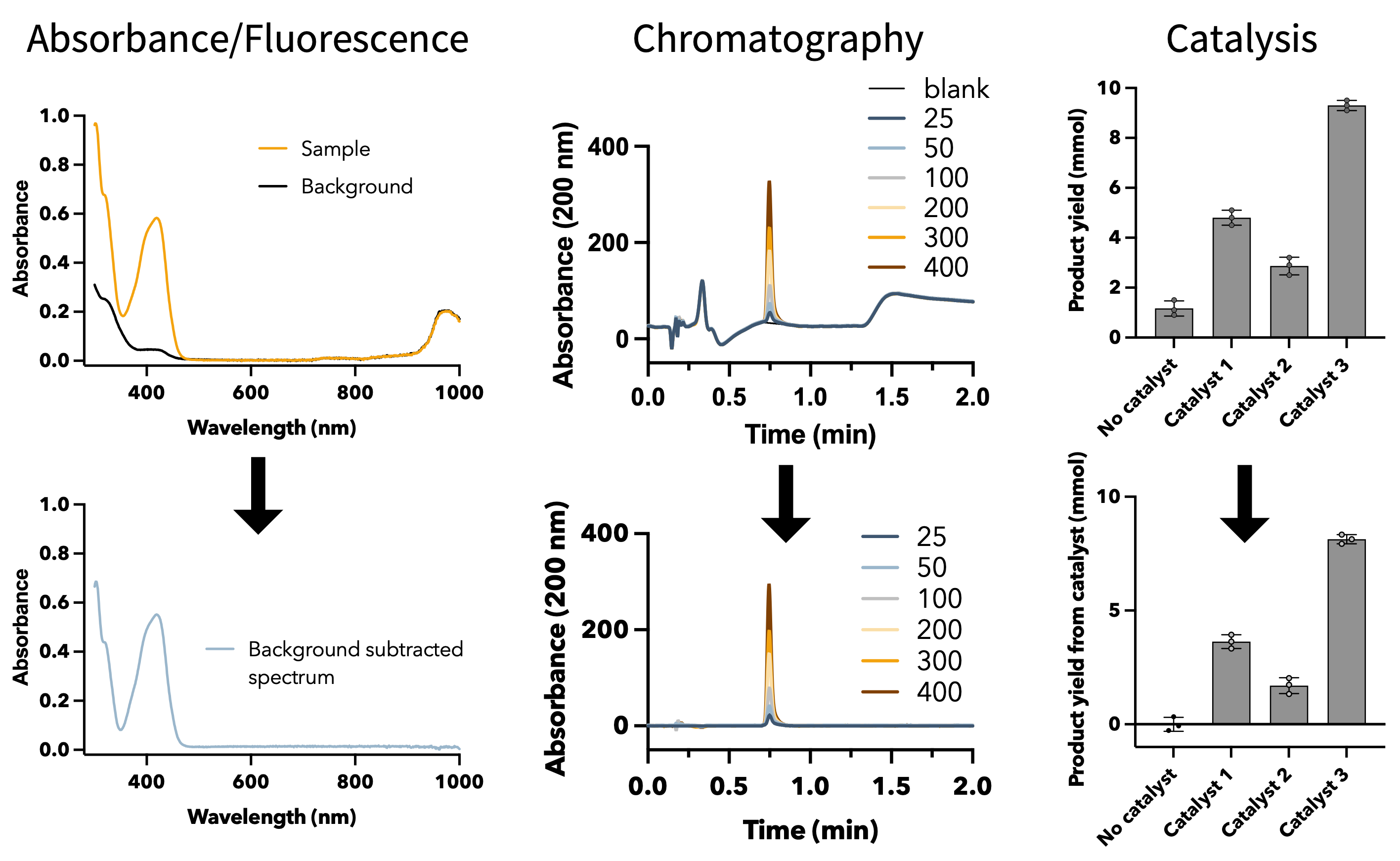
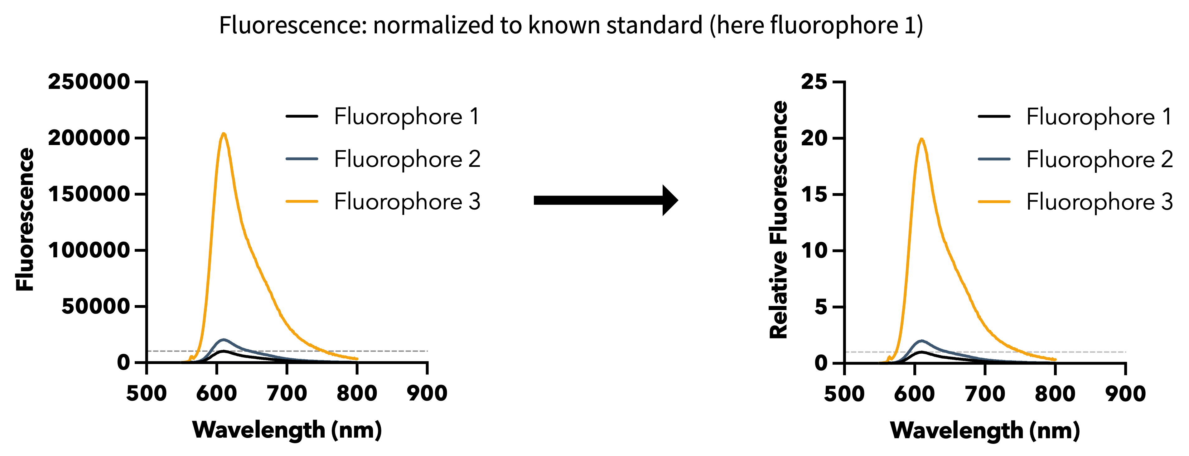
Standard normalization: divides by a reference value (e.g. catalyst concentration, maximum signal) to enable fair comparisons across conditions.

“Normalization” and “standardization” are used inconsistently across fields. In this course, the following distinction applies:

Standard normalization: dividing by a specific reference value meaningful to the domain (e.g. catalytic activity per mg of enzyme)
Min-max scaling: rescaling all values to the range [0, 1]: \(x' = (x - x_{\min}) / (x_{\max} - x_{\min})\). Useful for combining variables with different units. Sensitive to outliers.
Z-score standardization: subtracting the mean and dividing by the standard deviation: \(z = (x - \bar{x}) / s\). Centers the data at zero with unit variance. Very common in machine learning (preprocessing for PCA, linear regression with multiple inputs).

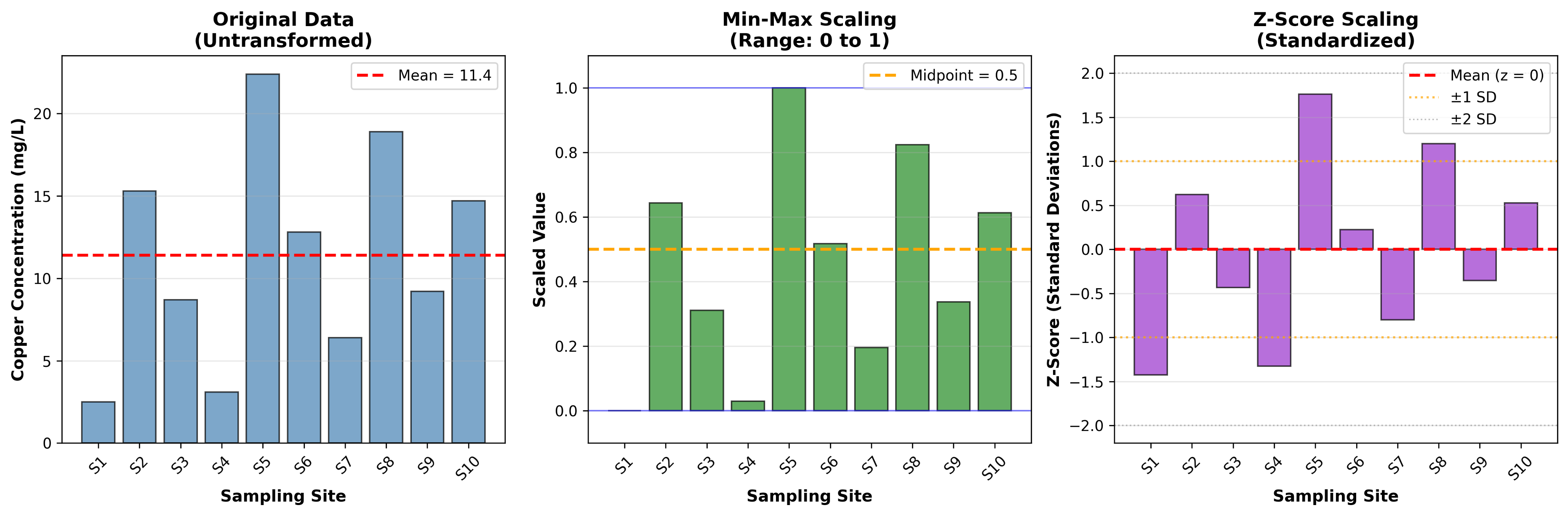
Z-score standardization is particularly important in PCA (Session 24) because features with larger ranges would otherwise dominate the first principal components.

Sometimes, both background subtraction and normalization are necessary to work up a dataset.

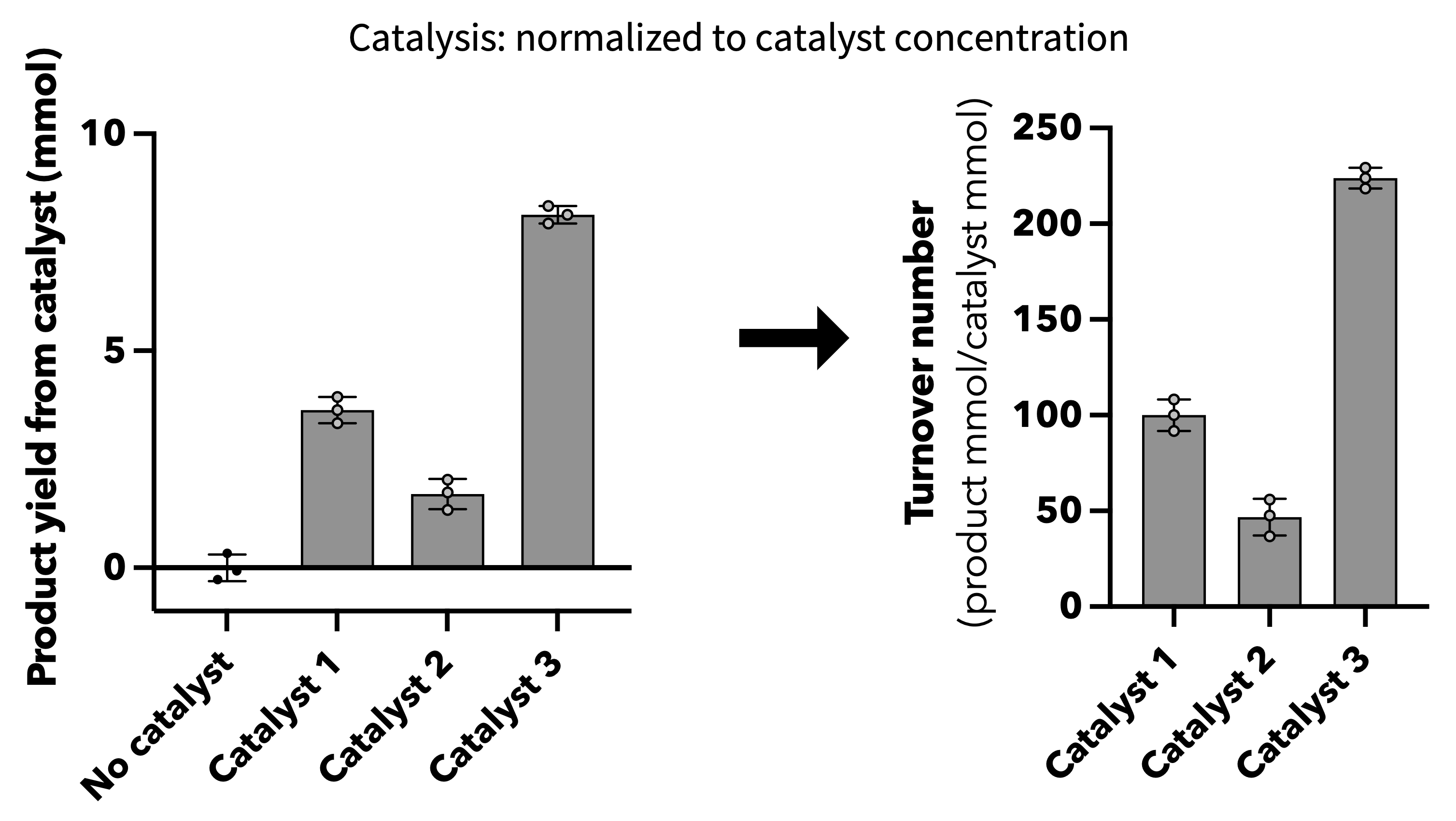
Note: we will discuss more complex data transformations when we get to regression analysis.

Common data transformations in Python

Background subtraction

Remove a blank/baseline signal to isolate the true signal:

normalizations

Standard normalization

Rescales data to mean = 0, standard deviation = 1. Required before PCA (Session 24):

Z-score standardization

Rescales data to mean = 0, standard deviation = 1. Required before PCA (Session 24):

Note: there are also tools to do z-scoring, but here we did it manually.

Min-max scaling

Rescales all values to the range [0, 1]:

Comparing the different normalizations

When to apply:

Background subtraction: Use when a blank/control measurement captures assay noise that applies equally to all samples.
Standard normalization: When a comparison to a known standard is necessary for clear interpretation.
Z-score standardization: When comparing/combining variables measured in different units (often the case in PCA or many ML tasks). Creates normally distributed data if the original is approximately normal.
Min-max scaling: Use when you need values bounded between 0 and 1 and are not concerned about outlier sensitivity. Skews the data distribution.

An Overall Statistical Analysis Workflow when x is discrete or categorical data

Define research question and hypotheses
Design the experiment (controls and replicates)
Collect the data
Visualize the data and transform if necessary
Determine descriptive statistics and error metrics
Assess normality
If normal, test variance. If non-normal, test for outliers (if any are removed, re-assess normality and variance, but do NOT detect outliers again)
Assess inferential statistics (including power and effect size)
Visualize data with inferential statistics
Formulate conclusions
Report methods, results, and conclusions

In later sessions, we will create parallel workflows for data with continuous input variables (correlation, regression).

Key takeaways

Identify outliers with IQR fences, Grubbs, or the MAD rule (robust to multiple outliers / masking).
Remove outliers only with documented justification; re-check assumptions afterward and do not re-detect.
Common transforms: background subtraction, min–max scaling, and z-score (required before PCA).
In Python: pg.madmedianrule(...), mark with np.nan, then StandardScaler (z-score) or min–max scaling.

In Person

TBD